Mean-field prediction for and simulation of a simple E-I network

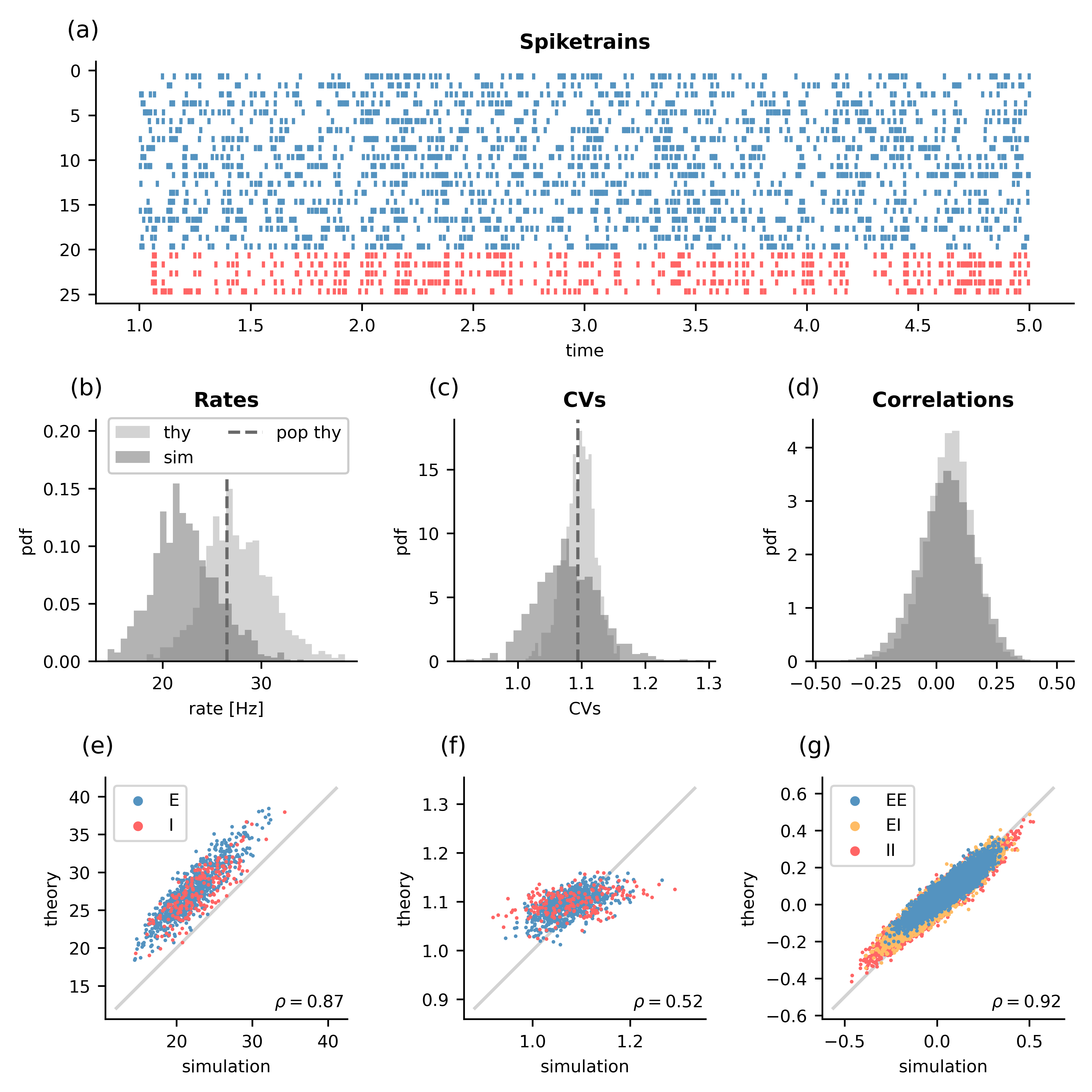
Fig. 1: Plot produced by this script showing a comparison of mean-field prediction and simulation results. (a) Spiketrains of 20 randomly chosen excitatory (blue) and 5 inhibitory (red) neurons. (b) Rates as predicted by single-neuron resolved mean-field theory (thy), from standard population resolved mean-field theory (pop thy), and the simulation (sim). (c) The same for the CVs. (d) The same for the pair-wise correlations. (e) The simulated rates vs. the rates predicted by single-neuron resolved mean-field theory for excitatory (E) and inhibitory (I) neurons. (f) The same for the CVs. (g) The same for the correlations, but separated by the different types of connections.

Here we show how to use NNMT to predict the results of a simulation of a simple E-I network with an excitatory (E) and an inhibitory (I) population of LIF neurons. The example was adapted from the code published with Layer et al. [2023], where the NEST simulation was based on the NEST example file brunel_exp_multisynapse_nest.py from NEST v3.4, which is free software under the terms of the GNU General Public License version 3.

First, a network is created using the simulation platform NEST [Gewaltig and Diesmann, 2007]. The connectivity matrix is then extracted to be used with NNMT. This allows computing the firing rates, CVs, and pairwise correlations with single-neuron resolved mean-field theory. We also compute the predictions of standard population resolved mean-field theory, which does not require the explicit realization of the connectivity matrix. Following that, we run the NEST simulation and compute the firing rates, CVs, and pairwise spike count correlations. Finally, we plot a comparison of all results in Fig. 1.

The network parameters are defined in network_params.yaml, the simulation parameters in simulation_params.yaml, and the analysis parameters in analysis_params.yaml.

We can see from Fig.1a that the network is in a asynchronous irregular state with somewhat bursty neurons. Furthermore, the simulated network is very small (800 excitatory, 200 inhibitory neurons), which introduces correlations due to shared inputs between the neurons that mean-field theory does not account for. Taken together, we expect mean-field theory to give reasonable predictions with slight deviations from the simulation. Under which conditions mean-field theory and simulation coincide is discussed in detail in Appendix D of Layer et al. [2023].

Note that NEST uses non SI units as standards, while NNMT uses SI units. This actually is one of the main difficulties when dealing with both software packages simultaneously.

Imports

import string
import matplotlib.pyplot as plt
import nest
import random
import numpy as np
import nnmt

Definition of config files, constants, and plotting options

network_param_file = 'config/network_params.yaml'
sim_param_file = 'config/simulation_params.yaml'
analysis_param_file = 'config/analysis_params.yaml'

network_id = 'ei_network'

# sample size for pair-wise correlations
sample_size = 10000

# plotting options
fontsize = 8
panel_label_fontsize = 11
labelsize = 8
markerscale = 5

# width and height of plot in mm
width = 180
height = 180

# colors used in plots
blue = '#5493C0'
red = '#FF6565'
yellow = '#FFBC65'
neutral = 'darkgray'
darkneutral = 'dimgray'

Functions

The script starts with the definition of all the functions used. The main script starts below.

Functions for creating the connectivity

def adjust_weights(neurons, W):
    """
    Sets the connectivity matrix W, but same connections need to exist already.
    """
    syn_collection = nest.GetConnections(neurons)
    targets = np.array([t for t in syn_collection.targets()]) - 1
    sources = np.array([s for s in syn_collection.sources()]) - 1
    syn_collection.set({'weight': W[targets, sources]})


def connectivity(neurons):
    """ Retrieves connectivity matrix from nest simulation """
    J = np.zeros((len(neurons), len(neurons)))
    syn_collection = nest.GetConnections(neurons)
    # get all targets, sources, and weights
    targets = np.array([t for t in syn_collection.targets()]) - 1
    sources = np.array([s for s in syn_collection.sources()]) - 1
    weights = np.array(syn_collection.get('weight'))

    # check for multapses
    # sort such that equal connections are next to each other
    idx = np.lexsort((sources, targets))
    targets = targets[idx]
    sources = sources[idx]
    weights = weights[idx]

    # calculate difference of subsequent elements and get position of zeros
    comb = np.vstack((targets, sources)).T
    mask = (np.diff(comb, axis=0) == [0, 0]).all(axis=1)
    mask = np.append(mask, [False])
    multapse_idx = np.where(mask)[0]

    # if multapses exist
    if len(multapse_idx) != 0:

        # split seperate connections
        split_idx = np.where(np.diff(multapse_idx) != 1)[0] + 1
        multapse_idx = np.split(multapse_idx, split_idx)

        # combine consecutive contributions: run over multapses and replace
        # multapse by respective single connection
        for m in multapse_idx:
            m = np.append(m, m[-1] + 1)
            weights[m[0]] = weights[m].sum()
            targets = np.delete(targets, m[1:])
            sources = np.delete(sources, m[1:])
            weights = np.delete(weights, m[1:])

    # get respective connectivity matrix
    J[targets, sources] = weights

    return J

Functions for extracting the simulation data

def get_spike_trains(senders, times, id_min, id_max):
    """Returns a list of spike trains sorted by senders."""
    sorted_ids = np.lexsort([times, senders])
    senders = senders[sorted_ids]
    times = times[sorted_ids]
    spike_trains = np.split(times, np.where(np.diff(senders))[0]+1)
    missing_senders = (set(np.arange(id_min, id_max + 1))
                       - set(np.unique(senders)))
    for id in sorted(missing_senders):
        spike_trains = (
            spike_trains[:id-id_min]
            + [np.array([])] + spike_trains[id-id_min:])
    return spike_trains

Functions for analyzing the simulation data

def bin_spiketrains(spiketrains, t_min, t_max, bin_width):
    """
    Bins the spiketrains from `t_min` to `t_max` with bin size `bin_width`.
    """
    bins = np.arange(t_min, t_max + bin_width, bin_width)
    clipped_spiketrains = [st[st < t_max] for st in spiketrains]
    clipped_spiketrains = [st[st >= t_min] for st in clipped_spiketrains]
    binned_spiketrains = np.array(
        [np.histogram(st, bins)[0] for st in clipped_spiketrains]
    )
    return binned_spiketrains


def remove_and_shift_init_from_spiketrains(spiketrains, T_init=0):
    """
    Remove initialization time from spiketrains and shift them respectively.
    """
    return [st[st >= T_init] - T_init for st in spiketrains]


def remove_inactive_neurons(spiketrains):
    """
    Remove all neurons for which an CV could not be calculated.

    This are all neurons which fired no more than 2 spikes.
    """
    nspikes = np.array([len(st) for st in spiketrains])
    return [spiketrains[id] for id in np.where(nspikes >= 3)[0]]


def get_spike_count_covariances(binned_spiketrains):
    """Computes the covariances of binned spiketrains."""
    return np.cov(binned_spiketrains)


def spectral_bound(matrix):
    """Computes the maximum real part of the eigenvalues of a given matrix."""
    return np.linalg.eigvals(matrix).real.max()


def calc_rates(spiketrains, T, T_init=0):
    """
    Calculates single neuron rates from spiketrains

    Parameters
    ----------
    spiketrains : list
        list of recorded spiketimes
    T : float
        Total simulation time including initialization in ms
    T_init : float
        Initialization time in ms

    Results
    -------
    array
        Rates in Hz
    """
    T -= T_init
    clipped_spiketrains = [st[st >= T_init] for st in spiketrains]
    rates = np.array([len(st) / T for st in clipped_spiketrains])
    return rates


def calc_isis(spiketrains):
    """
    Calculates the inter-spike-intervals.
    """
    return [np.diff(st) for st in spiketrains]


def calc_cvs(spiketrains):
    """
    Calculates the coefficients of variation of interspike intervals.
    """
    isis = calc_isis(spiketrains)
    stds = np.array([isi.std() for isi in isis])
    means = np.array([isi.mean() for isi in isis])
    return stds / means


def sample_corrs(data, sample_ixs):
    """
    Sample the correlation data for three different types of connections.
    """
    return data[(sample_ixs[0])], data[(sample_ixs[1])], data[(sample_ixs[2])]

Functions for plotting

def mm2inch(x):
    return x / 25.4


def add_panel_labels(axs, labels,
                     x_positions=None, y_positions=None,
                     fontsize=11, weight='normal', use_parenthesis=False):
    """
    Add panel labels. Default to standard position (-0.1, 1.1).
    """
    if use_parenthesis:
        labels = [f'({l})' for l in labels]
    if x_positions is None:
        x_positions = [-0.1] * len(axs)
    if y_positions is None:
        y_positions = [1.1] * len(axs)
    for n, ax in enumerate(axs):
        ax.text(x_positions[n], y_positions[n], labels[n],
                transform=ax.transAxes, size=fontsize, weight=weight)


def remove_borders(axs):
    for ax in axs:
        ax.spines['top'].set_visible(False)
        ax.spines['right'].set_visible(False)


def scatter_plot(ax, data1, data2, s=0.5, diag=True, set_aspect=True,
                 **kwargs):
    ax.scatter(data1, data2, s=s, **kwargs)
    if diag:
        lower, upper = get_extrema([data1, data2])
        plot_diagonal(ax, lower, upper)
    if set_aspect:
        ax.set_aspect('equal', 'box')


def get_extrema(datasets):
    lower = min([data.min() for data in datasets])
    upper = max([data.max() for data in datasets])
    return lower, upper


def plot_diagonal(ax, lower, upper, color='black', zorder=-100, **kwargs):
    lower -= 0.1 * (upper - lower)
    upper += 0.1 * (upper - lower)
    diagonal = np.linspace(lower, upper)
    ax.plot(diagonal, diagonal, color=color, zorder=zorder, **kwargs)


def add_corrcoef(ax, cc, x=0.7, y=0.05):
    ax.text(x, y, f'$\\rho={cc:.2g}$', transform=ax.transAxes)


def plot_rates_scatter_plot(ax_rates, rates_sim, rates_thy, cc_rate, N_E):

    lower, upper = get_extrema([rates_sim, rates_thy])
    plot_diagonal(ax_rates, lower, upper, color='lightgray')
    scatter_plot(ax_rates, rates_sim[:N_E], rates_thy[:N_E], color=blue,
                 label='E', diag=False, rasterized=True)
    scatter_plot(ax_rates, rates_sim[N_E:], rates_thy[N_E:], color=red,
                 label='I', diag=False, rasterized=True)
    add_corrcoef(ax_rates, cc_rate)


def plot_corrs_scatter_plot(ax_corrs,
                            corrs_sim_EE, corrs_sim_EI, corrs_sim_II,
                            corrs_thy_EE, corrs_thy_EI, corrs_thy_II,
                            cc_corr):

    lower, upper = get_extrema([corrs_sim_EE, corrs_thy_EE,
                                corrs_sim_EI, corrs_thy_EI,
                                corrs_sim_II, corrs_thy_II])
    plot_diagonal(ax_corrs, lower, upper, color='lightgray')
    scatter_plot(ax_corrs, corrs_sim_EE, corrs_thy_EE, diag=False,
                 color=blue, label='EE', rasterized=True,
                 zorder=3)
    scatter_plot(ax_corrs, corrs_sim_EI, corrs_thy_EI, diag=False,
                 color=yellow, label='EI', rasterized=True,
                 zorder=2)
    scatter_plot(ax_corrs, corrs_sim_II, corrs_thy_II, diag=False,
                 color=red, label='II', rasterized=True,
                 zorder=1)
    add_corrcoef(ax_corrs, cc_corr)


def raster_plot(ax, spiketrains, samples=[20, 5], t_min=1, t_max=5,
                colors=['steelblue', 'red'], marker='ticks', **kwargs):
    slices = np.append([0], np.array(samples)).cumsum()
    for i in range(len(samples)):
        sts = random.choices(spiketrains[i], k=samples[i])
        sts = [st[(st > t_min) & (st < t_max)] for st in sts]
        neuron_ids = np.arange(slices[i], slices[i+1])
        for id, spiketrain in zip(neuron_ids + 1, sts):
            if marker == 'ticks':
                ax.scatter(spiketrain, id * np.ones(len(spiketrain)),
                        color=colors[i], marker=2, s=8, **kwargs)
            elif marker == 'dots':
                ax.scatter(spiketrain, id * np.ones(len(spiketrain)),
                        color=colors[i], s=0.5, **kwargs)
            else:
                raise RuntimeError(f'Marker {marker} unknown.')
    ax.set_ylim([slices[-1]+1, -1])

Drawing a connectivity matrix with NEST

First, we must draw a random connectivity matrix using NEST.

We start by loading the parameters from the yaml files in which we used the units that NEST is expecting. We load the parameters in these units here. Time constants such as tau_m, for example, are given in ms.

network_params = nnmt.input_output.load_val_unit_dict_from_yaml(
    network_param_file)
nnmt.utils._strip_units(network_params)

sim_params = nnmt.input_output.load_val_unit_dict_from_yaml(
    sim_param_file)
nnmt.utils._strip_units(sim_params)

Next, we define the parameters for building the network.

connection_rule = network_params['connection_rule']
multapses = network_params['multapses']
neuron_type = network_params['neuron_type']
gaussianize = network_params['gaussianize']

N_E = network_params['N'][0]  # number of excitatory neurons
N_I = network_params['N'][1]  # number of inhibitory neurons
N = network_params['N'].sum()  # number of neurons in total

p = network_params['p']  # connection probability
K_E = int(p * N_E)  # number of excitatory synapses per neuron
K_I = int(p * N_I)  # number of inhibitory synapses per neuron

tau_m = network_params['tau_m']  # time const of membrane potential in ms
tau_r = network_params['tau_r']  # refactory time in ms
tau_s = network_params['tau_s']  # synaptic time constant in ms
delay = network_params['d']  # synaptic delay in ms

V_r = network_params['V_0_rel']  # reset potential in mV
V_th = network_params['V_th_rel']  # membrane threshold potential in mV
V_m = network_params['V_m']  # initial potential in mV
E_L = network_params['E_L']  # resting potential in mV

g = network_params['g']  # absolute ratio inhibitory weight/excitatory weight
J = network_params['j']  # postsynaptic amplitude in mV
J_ex = J  # amplitude of excitatory postsynaptic current in mV
J_in = -g * J_ex  # amplitude of inhibitory postsynaptic current in mV

p_rate_E = network_params['nu_ext'][0]  # external excitatory noise rate in Hz
p_rate_I = network_params['nu_ext'][1]  # external inhibitory noise rate in Hz
I_ext = network_params['I_ext']  # external DC current in pA

C = network_params['C']  # membrane capacitance in pF

The parameters of the neurons are stored in a dictionary. If the neurons have exponential synapses, the synaptic time constant is defined as well.

neuron_params = {
    "C_m": C,
    "tau_m": tau_m,
    "t_ref": tau_r,
    "E_L": E_L,
    "V_reset": V_r,
    "V_m": V_m,
    "V_th": V_th,
    "I_e": I_ext
    }

if neuron_type == 'iaf_psc_exp':
    neuron_params['tau_syn_ex'] = tau_s
    neuron_params['tau_syn_in'] = tau_s

Then, we configure the NEST simulation kernel. We need to set these properties here, since we want to simulate the network afterwards. They cannot be modified after NEST nodes have been created, which we need to do in order to draw the connectivity matrix.

nest.ResetKernel()
nest.local_num_threads = sim_params['local_num_threads']
nest.resolution = sim_params['dt']

Here, we create the NEST nodes.

print("Building network")

if neuron_type == 'iaf_psc_delta':
    nodes_ex = nest.Create("iaf_psc_delta", N_E, params=neuron_params)
    nodes_in = nest.Create("iaf_psc_delta", N_I, params=neuron_params)
elif neuron_type == 'iaf_psc_exp':
    nodes_ex = nest.Create("iaf_psc_exp", N_E, params=neuron_params)
    nodes_in = nest.Create("iaf_psc_exp", N_I, params=neuron_params)
neurons = nodes_ex + nodes_in

For connecting the network, we need to define the synapse properties.

nest.CopyModel("static_synapse", "excitatory",
               {"weight": J_ex, "delay": delay})
nest.CopyModel("static_synapse", "inhibitory",
               {"weight": J_in, "delay": delay})

syn_params_ex = {"synapse_model": "excitatory"}
syn_params_in = {"synapse_model": "inhibitory"}

Here, we seed the random number generators. This might seem like an odd place to do this, but we noticed that if the seed is defined further above, it is reset for some reason we do not understand.

np.random.seed(sim_params['np_seed'])
nest.rng_seed = sim_params['seed']

Next, we connect the different nodes using some NEST connection rule. This is the point were the connectivity matrix is drawn.

print("Connecting network")

if connection_rule == 'pairwise_bernoulli':
    conn_params_ex = {'rule': 'pairwise_bernoulli', 'p': p,
                    'allow_multapses': multapses}
    conn_params_in = {'rule': 'pairwise_bernoulli', 'p': p,
                    'allow_multapses': multapses}
elif connection_rule == 'fixed_indegree':
    conn_params_ex = {'rule': 'fixed_indegree', 'indegree': K_E,
                    'allow_multapses': multapses}
    conn_params_in = {'rule': 'fixed_indegree', 'indegree': K_I,
                    'allow_multapses': multapses}
else:
    raise ValueError(f'Connection rule {connection_rule} not implemented!')

print("Excitatory connections")
nest.Connect(nodes_ex, nodes_ex + nodes_in, conn_params_ex, syn_params_ex)

print("Inhibitory connections")
nest.Connect(nodes_in, nodes_ex + nodes_in, conn_params_in, syn_params_in)

Then, we can extract the connectivity matrix using our custom function.

print("Extracting connectivity matrix")
W = connectivity(neurons)

Here, we “Gaussianize” the connectivity matrix. We introduced this because mean-field theory predicts the same values for all firing rates and many other attributes if the synaptic weights of all connections are identical and each neuron receives a set number of inputs (as is the case for the connection rule fixed_indegree). To get around this, we chose to use a richer type of connectivity in our example.

if gaussianize:
    print("Gaussianizing connectivity matrix")
    J_std = network_params['j_std'] * np.abs(J_ex)

    W[W != 0] += np.random.normal(
        loc=0, scale=J_std, size=np.count_nonzero(W))

    adjust_weights(neurons, W)

Prediction using NNMT

Single-neuron resolved mean-field theory

Now that we have the connectivity matrix, we want to predict the single-neuron resolved rates, CVs and pairwise correlations using NNMT.

We start by building a NNMT network. This time the parameter units are directly converted to SI units. We add the newly created connectivity matrix J, the respective - and here trivial - indegree matrix K, as well as their external counterparts J_ext and K_ext to the network parameters. Here, we need to pay attention to convert everything to the right units.

print('Build NNMT model')

network = nnmt.models.Plain(network_param_file)

# Add newly calculated parameters to network parameter dictionary
new_network_params = dict(
    K=np.where(W != 0, 1, 0),  # here we assume that multapses are not allowed!
    J=W/1000,  # convert from mV to V
    K_ext=np.vstack([np.ones(N), np.ones(N)]).T,
    J_ext=np.vstack([np.ones(N) * J_ex, np.ones(N) * J_in]).T / 1000  # mV to V
)

network.network_params.update(new_network_params)

# This is just to ensure that the synaptic time constant is set correctly, even
# if the synaptic time constant is defined in the yaml file.
if neuron_type == 'iaf_psc_delta':
    network.network_params['tau_s'] = 0.0

Computing the rates, CVs, and correlations is just a matter of calling a few functions now. Note that we are using functions for LIF neurons with exponential synapses despite using a NEST neuron type with delta synapses. However, this yields correct results if the synaptic time constant is set to zero in the network parameters.

print('Estimate firing rates')
working_point = nnmt.lif.exp.working_point(network)
rates_thy = working_point['firing_rates']

print('Estimate CVs')
cvs_thy = nnmt.lif.exp.cvs(network)

print('Estimate effective connectivity')
W_eff = nnmt.lif.exp.pairwise_effective_connectivity(network)

print('Estimate pairwise covarianes and correlations')
covs_thy = nnmt.lif.exp._pairwise_covariances(W_eff, rates_thy, cvs_thy)
std_thy = np.sqrt(np.diag(covs_thy))
corrs_thy = covs_thy / np.outer(std_thy, std_thy)

Population resolved mean-field theory

We also want to compute the standard mean-field predictions for the two populations. Therefore we create another NNMT model, where the connectivity matrix J now is the synaptic weight matrix. The indegree matrix K and the external counterparts J_ext and K_ext need to be defined again.

print('Build NNMT population model')

K_pop = np.array([[K_E, K_I], [K_E, K_I]])
J_pop = np.array([[J_ex, J_in],
                    [J_ex, J_in]])
# convert from mV to V
J_pop /= 1000

K_ext_pop = np.array([[1, 1],
                        [1, 1]])
J_ext_pop = np.array([[J_ex, J_in],
                        [J_ex, J_in]])
# convert from mV to V
J_ext_pop /= 1000

pop_network = nnmt.models.Plain(network_param_file)
pop_network.network_params['K'] = K_pop
pop_network.network_params['J'] = J_pop
pop_network.network_params['K_ext'] = K_ext_pop
pop_network.network_params['J_ext'] = J_ext_pop

For calculating the rates and CVs we again only need to call a few functions. Note that the pairwise correlations cannot be computed in population resolved mean-field theory, which would only allow to compute mean correlations, but this has not been implemented in NNMT yet.

print('Estimate population rates')
nnmt.lif.exp.working_point(pop_network)
rates_pop = nnmt.lif.exp.firing_rates(pop_network)

print('Estimate population CVs')
cvs_pop = nnmt.lif.exp.cvs(pop_network)

Simulating the network

Finally, we want to simulate the network using NEST. Therefore, we need to finish preparing NEST.

First, we create the missing nodes, namely the recorders and external inputs. We could not create them before extracting the connectivity matrix since our algorithm would have misinterpreted them as neurons, resulting in an incorrect connectivity matrix.

spike_recorder = nest.Create("spike_recorder")

noise_E = nest.Create("poisson_generator", params={"rate": p_rate_E})
noise_I = nest.Create("poisson_generator", params={"rate": p_rate_I})

We connect the missing devices.

print("Connecting devices")
nest.Connect(nodes_ex + nodes_in, spike_recorder,
            syn_spec="excitatory")

nest.Connect(noise_E, nodes_ex + nodes_in, syn_spec=syn_params_ex)
nest.Connect(noise_I, nodes_ex + nodes_in, syn_spec=syn_params_in)

And finally, we simulate the network

print("\nStart simulation")
simtime = sim_params['simtime']  # simulation time in ms
nest.Simulate(simtime)
print("\nSimulation finished")

and extract the spiketrains.

print('Extract spiketrains')
spiketrains = []
events = spike_recorder.get('events')
times = events['times']
senders = events['senders']
id_min = 1
id_max = N
spiketrains = get_spike_trains(senders, times, id_min, id_max)

Analyzing the simulation data

Here, we compute the firing rates, CVs, and pairwise correlations from the simulation data.

First, we load the analysis parameters.

print('Analyze simulation results')

analysis_params = nnmt.input_output.load_val_unit_dict_from_yaml(
    analysis_param_file)
nnmt.utils._convert_to_si_and_strip_units(analysis_params)

T_init = analysis_params['T_init']
binwidth = analysis_params['binwidth']

Then, we compute the properties using our custom functions.

# convert units to SI units (from ms to s)
simtime = sim_params['simtime'] / 1000
spiketrains = [st / 1000 for st in spiketrains]

# remove initialization time
clipped_spiketrains = remove_and_shift_init_from_spiketrains(
    spiketrains, T_init)

# calculate rates
print('Calculate simulated rates')
rates_sim = calc_rates(spiketrains, simtime, T_init)

# calculate cvs
print('Calculate simulated CVs')
cvs_sim = calc_cvs(clipped_spiketrains)

print('Calculate simulated correlations')
binned_spiketrains = bin_spiketrains(
    spiketrains, T_init, simtime, binwidth)
corrs_sim = np.corrcoef(binned_spiketrains)

Separating results into different populations and subsampling

In order to plot the data, we need to divide them into the different populations (E, I), and the different types of connections (EE, EI, II). Furthermore, we pick a subset of the spiketrains and the pair-wise correlations for plotting since otherwise there would be too many data points.

print('Separate population results')

# separate spiketrains into E and I

random.seed(42)
spiketrains_E = random.choices(spiketrains[:N_E], k=75)
spiketrains_I = random.choices(spiketrains[N_E:], k=25)

# separate and subsample correlations

ix = np.triu_indices_from(corrs_thy, k=1)

cross_corrs_sim = corrs_sim[ix]
cross_corrs_thy = corrs_thy[ix]

ix = np.array(ix)
ix_EE = ix[:, (ix[0] < N_E) & (ix[1] < N_E)]
ix_EI = ix[:, (ix[0] < N_E) & (ix[1] >= N_E)]
ix_II = ix[:, (ix[0] >= N_E) & (ix[1] >= N_E)]
ixs = [ix_EE, ix_EI, ix_II]

np.random.seed(42)
sample_ixs = []
for ix in ixs:
    sample_ix = np.random.choice(
        np.arange(len(ix[0])), size=sample_size, replace=False)
    sample_ixs.append((ix[0][sample_ix], ix[1][sample_ix]))

corrs_thy_EE, corrs_thy_EI, corrs_thy_II = sample_corrs(corrs_thy, sample_ixs)
corrs_sim_EE, corrs_sim_EI, corrs_sim_II = sample_corrs(corrs_sim, sample_ixs)

sampled_cross_corrs_thy = np.append(corrs_thy_EE, [corrs_thy_EI, corrs_thy_II])
sampled_cross_corrs_sim = np.append(corrs_sim_EE, [corrs_sim_EI, corrs_sim_II])

Plotting of results

Finally, we plot Fig. 1.

print('Start plotting')

width = mm2inch(width)
height = mm2inch(height)

fig = plt.figure(figsize=[width, height])

plt.rc('font', size=fontsize)
plt.rc('xtick', labelsize=labelsize)
plt.rc('ytick', labelsize=labelsize)

grid = (3, 3)

cc_rates = np.corrcoef(rates_sim, rates_thy)[0, 1]
cc_cvs = np.corrcoef(cvs_sim, cvs_thy)[0, 1]
cc_corrs = np.corrcoef(cross_corrs_sim, cross_corrs_thy)[0, 1]

ax_spiketrains = plt.subplot2grid(grid, (0, 0), colspan=3)
ax_rates_hist = plt.subplot2grid(grid, (1, 0))
ax_cvs_hist = plt.subplot2grid(grid, (1, 1))
ax_corrs_hist = plt.subplot2grid(grid, (1, 2))
ax_rates = plt.subplot2grid(grid, (2, 0))
ax_cvs = plt.subplot2grid(grid, (2, 1))
ax_corrs = plt.subplot2grid(grid, (2, 2))
axs = [ax_spiketrains,
       ax_rates_hist, ax_cvs_hist, ax_corrs_hist,
       ax_rates, ax_cvs, ax_corrs]


print('Plot spiketrains')
raster_plot(ax_spiketrains,
            [spiketrains_E, spiketrains_I],
            colors=[blue, red])
ax_spiketrains.set_title('Spiketrains', fontweight='bold')
ax_spiketrains.set_xlabel('time')


print('Plot histograms')
hist1 = ax_rates_hist.hist(rates_thy, bins=30, alpha=0.5, density=True,
                   label='thy',
                   color=neutral)
hist2 = ax_rates_hist.hist(rates_sim, bins=30, alpha=0.5, density=True,
                   label='sim',
                   color=darkneutral)
ax_rates_hist.set_title('Rates', fontweight='bold')
ax_rates_hist.set_ylim([0,0.21])
ax_rates_hist.set_xlabel('rate [Hz]')
ax_rates_hist.set_ylabel('pdf')
line = ax_rates_hist.axvline(rates_pop.mean(),
                      label='pop thy',
                      color='dimgrey',
                      linestyle='--')
#get handles and labels
handles, labels = ax_rates_hist.get_legend_handles_labels()

#specify order of items in legend
order = [1, 2, 0]

#add legend to plot
ax_rates_hist.legend(
    [handles[idx] for idx in order],[labels[idx] for idx in order],
    ncol=2, framealpha=1, bbox_to_anchor=(1, 1.04), loc='upper right')

ax_cvs_hist.hist(cvs_thy, bins=30, alpha=0.5, density=True, color=neutral)
ax_cvs_hist.hist(cvs_sim, bins=30, alpha=0.5, density=True, color=darkneutral)
ax_cvs_hist.set_title('CVs', fontweight='bold')
ax_cvs_hist.set_xlabel('CVs')
ax_cvs_hist.set_ylabel('pdf')
ax_cvs_hist.axvline(cvs_pop.mean(), color='dimgrey', linestyle='--')

ax_corrs_hist.hist(sampled_cross_corrs_thy, bins=30, alpha=0.5, density=True,
                   color=neutral)
ax_corrs_hist.hist(sampled_cross_corrs_sim, bins=30, alpha=0.5, density=True,
                   color=darkneutral)
ax_corrs_hist.set_title('Correlations', fontweight='bold')
ax_corrs_hist.set_ylabel('pdf')


print('Plot scatter plots')
plot_rates_scatter_plot(ax_rates, rates_sim, rates_thy, cc_rates, N_E)
ax_rates.set_xlabel('simulation')
ax_rates.set_ylabel('theory')
plot_rates_scatter_plot(ax_cvs, cvs_sim, cvs_thy, cc_cvs, N_E)
ax_cvs.set_xlabel('simulation')
ax_cvs.set_ylabel('theory')
plot_corrs_scatter_plot(ax_corrs,
                        corrs_sim_EE, corrs_sim_EI, corrs_sim_II,
                        corrs_thy_EE, corrs_thy_EI, corrs_thy_II,
                        cc_corrs)
ax_corrs.set_xlabel('simulation')
ax_corrs.set_ylabel('theory')

ax_rates.legend(markerscale=markerscale)
leg = ax_corrs.legend(markerscale=markerscale)
for lh in leg.legendHandles:
    lh.set_alpha(1)

print('Formatting of figure')
labels = list(string.ascii_lowercase[:len(axs)])

x_positions = [-0.1] * len(axs)
x_positions[0] = -0.03

add_panel_labels(axs, labels, x_positions=x_positions,
                 fontsize=panel_label_fontsize,
                 use_parenthesis=True)
remove_borders(axs)

plt.tight_layout()
plt.savefig(network_id + '.png', dpi=600)
plt.close()