Binary rates: simulation vs mean-field

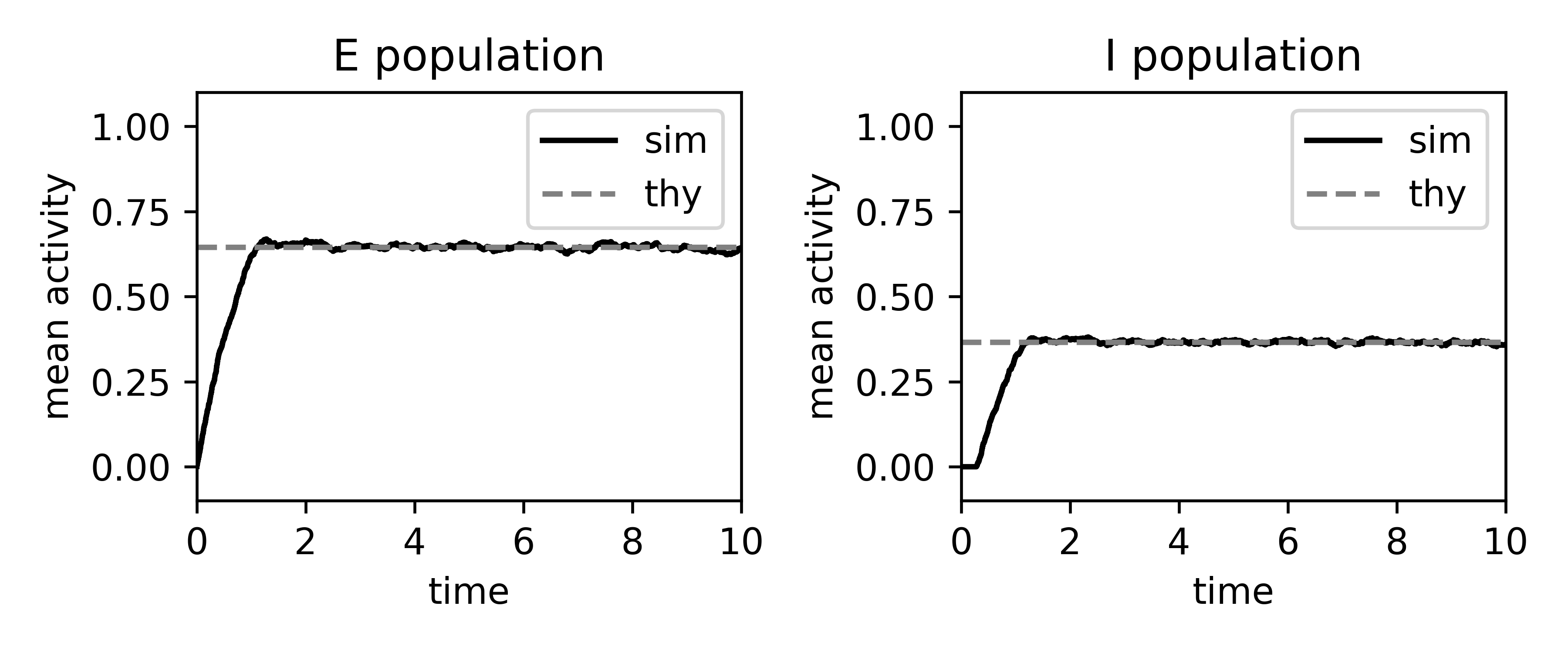
Here we simulate an E-I network of binary neurons, calculate the mean-field estimate of the firing rates, and plot them together.

import nnmt
import numpy as np
import matplotlib.pyplot as plt

Helper functions

First, we define the functions used to perform the simulation.

def _sort_queue(q):
    """
    Sorts a 2d array of id and update time point by update time points.

    Sorts the queue of update time points
        id_0, t_next_0
        id_1, t_next_1
        ...
    by the update time point t_next.

    Parameters
    ----------
    q : array
        2d array of neuron ids and update time points.

    Returns
    -------
    array
        Sorted array of ids and update time points.
    """
    return q[np.argsort(q[:, 1], kind='stable')]


def update_poisson(J, S, T, tau, thetas):
    """
    Simulates a network of binary neurons.

    Evolves the initial network state `S` in time by drawing exponentially
    distributed update times (Poisson process) with time constant `tau` until
    time `T` is reached, using connectivity matrix `J` and thresholds `thetas`.

    Parameters
    ----------
    J : array
        Connectivity matrix.
    S : array
        Initial state of each neuron.
    T : float
        Simulation time.
    tau : float
        Time constant of all binary neurons.
    thetas : [array|list]
        Thresholds of neurons.

    Returns
    -------
    array
        Update times.
    array
        State of each neuron at each update time point.
    array
        Mean population activity at each update time point.
    """
    # check dimensions of J and S
    assert J.shape[0] == J.shape[1] == S.shape[0]
    # get total number of neurons
    N = S.shape[0]
    # create update queue
    update_queue = np.empty((N, 2), dtype=np.float32)
    update_queue[:, 0] = np.arange(N)
    # draw first update time point for every neuron
    # from an exponential distribution with mean tau
    update_queue[:, 1] = np.random.exponential(tau, N)
    # sort queue ascendingly according to update time
    update_queue = _sort_queue(update_queue)
    # initialize storage lists
    ts, m, Ss = [], [], []
    t = 0
    while t < T:
        # select neuron with next update time point
        i, t = update_queue[0, :]
        i = int(i)
        # input to neuron i
        h_i = J[i, :].dot(S)
        # update state of neuron i
        S[i] = np.heaviside(h_i-thetas[i], 0)
        # draw new update time
        update_queue[0, 1] += np.random.exponential(tau)
        update_queue = _sort_queue(update_queue)
        m.append(S.mean())
        ts.append(t)
        Ss.append(S.copy())
    return np.array(ts), np.array(Ss).T, np.array(m)

Here we define the functions that construct the network properties in a format needed to perform the simulation.

def fixed_indegree_connectivity(N, J, K):
    """
    Constructs a fixed indegree matrix for the given network parameters.

    Parameters
    ----------
    N : array of ints
        Number of neurons in each population.
    J : array of floats
        Weight matrix.
    K : array of ints
        Indegree matrix.

    Returns
    -------
    array
        Connectivity matrix.
    """

    W = np.zeros((N.sum(), N.sum()), dtype=np.float32)

    # list of neurons (each one gets a unique number)
    neurons = np.arange(N.sum())

    population_ix = N.cumsum()

    for pre_ix, pre_pop in enumerate(
            np.array_split(neurons, population_ix[:-1])):
        for post_ix, post_pop in enumerate(
                np.array_split(neurons, population_ix[:-1])):
            for post_neuron in post_pop:
                pre_neurons = np.random.choice(pre_pop[pre_pop!=post_neuron],
                                               size=K[post_ix][pre_ix],
                                               replace=False)
                W[post_neuron, pre_neurons] = J[post_ix][pre_ix]

    return W


def neuron_thresholds(N, theta):
    """
    Creates a list of thresholds for each neuron.

    Parameters
    ----------
    N : array
        Numbers of neurons in each population.
    theta : array
        Threshold for each population

    Returns
    -------
    array
        Threshold for each individual neuron numbered from 0 to N-1.
    """
    thresholds = np.zeros(N.sum())
    population_ix = np.append([0], N.cumsum())
    for i in range(len(population_ix[:-1])):
        thresholds[population_ix[i]: population_ix[i+1]] = theta[i]
    return thresholds

Parameter definition

Here we define the network parameters

# numbers of neurons in each population and their respective name
N = np.array([1000, 1000])
label = ['E', 'I']

# indegree matrix
K = np.array([[150, 200],
              [350, 200]])

# weight matrix
J = np.array([[0.1, -0.2],
              [0.1, -0.2]])

network_params = {'J': J, 'K': K, 'N': N}

Calculation of mean-field estimate

Lets define the network model. We decided to use the Plain model, as we just want to load the parameters into the models dicts and do not want to calculate any dependent parameters from them.

# here we have to copy the dict due to a bug in ``nnmt.models.Network``
network = nnmt.models.Plain(dict(network_params))

We could set the firing threshold of the neurons directly, but here we decided to calculate the threshold using a balanced condition for some expected rates

expected_rates = [0.7, 0.4]
theta = nnmt.binary.balanced_threshold(network, expected_rates)
network.network_params['theta'] = theta

We calculate the mean-field estimate of the rates

rates_thy = nnmt.binary.mean_activity(network)

Simulation

For simulating the network we require a concrete realization of the network connectivity

W = fixed_indegree_connectivity(**network_params)

And we are going to use a list that defines the thresholds of each neuron separately

thresholds = neuron_thresholds(network.network_params['N'],
                               network.network_params['theta'])

The simulation additionally requires to define the time constant of the neurons

sim_params = {'tau': 1., 'thetas': thresholds}

Then we can run the simulation

# simulation time
T = 10
# initial state
S = np.zeros(W.shape[0], dtype=np.float32)
# simulate
t, S, m = update_poisson(W, S, T=T, **sim_params)

Now we calculate the mean rates for each population

rates_sim = np.array([pop.mean(axis=0)
                      for pop in np.array_split(S, N.cumsum()[:-1])])

Plotting

fig, axs = plt.subplots(1, len(N), figsize=(6, 2.5))
for i in range(len(N)):
    axs[i].plot(t, rates_sim[i], '-', color='k', label='sim')
    axs[i].plot(t, rates_thy[i]*np.ones_like(t), '--', color='gray',
                label='thy')
    axs[i].set_xlim(0, T)
    axs[i].set_ylim(-0.1, 1.1)
    axs[i].set_xlabel('time')
    axs[i].set_ylabel('mean activity')
    axs[i].legend(loc=0)
    axs[i].set_title(f'{label[i]} population')

plt.tight_layout()
plt.savefig('binary.png', dpi=600)
plt.show()